User Manual

Authors:

Guillaume Touya, Justin Berli, Azelle Courtial

Copyright:

This work is licensed under a European Union Public Licence v1.2.

Abstract:

This document explains how to use the CartAGen Python library for cartographic generalisation.

Introduction

The user manual aims at providing an overview of the cartographic generalisation algorithms proposed by CartAGen. Some complex algorithms and processes are more deeply explained here than in the API Reference, in particular for those having several steps.

This section is also designed to help you decide which algorithm best fit your needs. Indeed, several generalisation methods are developped to address the same issue, for example to avoid polygon cluttering or to simplify lines and polygons. Those issues can also depend on the type of geographic objects you are trying to generalise. For example, maybe you don’t want to simplify rivers and roads the same way, as their representation on the map doesn’t have the same constraints.

With that in mind, we tried here to offer an overview of the algorithms offered by CartAGen in order to help you make a choice in your cartographic endeavors. Please keep in mind that this is not a lecture on cartographic generalisation nor a full explanation of the generalisation process. We have designed several Jupyter notebooks to serve as learning material, they are accessible here.

This user manual also assumes you have a certain knowledge of the Python libraries Shapely and GeoPandas as CartAGen relies on those data format and geometry types. Furthermore, please ensure you are working with projected geographic data as the vast majority of generalisation tools provided by this library relies on spatial operations.

Points

Reduction

The reduction of points is a useful method to declutter the map. It can be used for several types of objects such as toponyms and symbols but can also be used to generate thematic maps from a really dense set of points.

K-Means, Quad Tree and Label Grid are 3 different algorithms to generate clusters of points. Aggregation, selection and simplification are 3 different methods for using those clusters and are aimed at different use cases.

K-Means-based algorithms :

• K-Means aggregation

• K-Means selection

• K-Means simplification

Quad Tree-based algorithms [1] :

• Quad Tree aggregation

• Quad Tree selection

• Quad Tree simplification

Label Grid-based algorithms [2] :

• Label Grid aggregation

• Label Grid selection

• Label Grid simplification

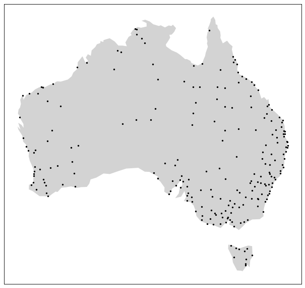
In this section, we will show those three algorithms on the Australian cities from Natural Earth because of their repartition on the island. Indeed, most Australian cities are localised on the southeastern coast of the country, which offers a good way to test the different point reduction algorithms to see how they keep the heterogeneity of the data.

(Source code)

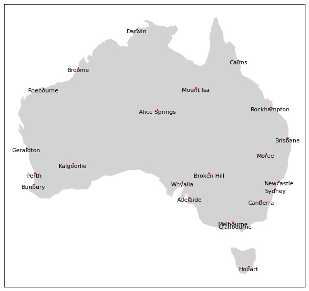
The Australian cities from Natural Earth designed for the 1:10m scale

The K-Means clustering algorithm can be used used to reduce the amount of points by forming clusters based on the spatial proximity of the cities. In selection mode, like the following image shows, only the city with the largest population are kept.

(Source code)

The Australian cities reduced by the K-Means method with a shrink ratio of 0.1 (10% of the cities are kept) and keeping the city with the largest population for each cluster.

On the other hand, the Quad Tree based algorithm in selection mode can be used for the same purpose. This method can be interesting to adress the same issue and is quicker as the amount of points is recursively divided while the quad tree depth rises.

(Source code)

World’s cities reduced using the Quad Tree method with a depth of 3 by selection on the largest population

Finally, the Label Grid algorithm can also be used in selection mode, like the Quad Tree, but uses a regular grid of a given size and shape.

(Source code)

World’s cities reduced using the Label Grid method with an hexagonal grid of 500,000x500,000 meters by selection on the largest population

Covering

Covering algorithms are used to transform points into surfaces. For now, two methods are available, which are:

• Delaunay convex and concave hull [3]

• Swinging arm algorithm [4]

The Delaunay method can only create a single polygon, thus, if you want to use this method, you should first generate clusters using the right library, such as scikit-learn clustering, and then create the hulls for each cluster. On the other hand, the swinging arm algorithm can create multiple polygons as can be seen on the following image.

(Source code)

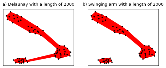
Comparison of the two covering methods

Heatmap

CartAGen also proposes a Heatmap [5] function to visualize the density of points within a dataset. For example, we can display the density of Australian cities weighted by the population.

(Source code)

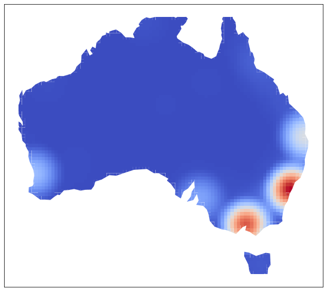
The density of cities in Australia weighted by the population

Lines

Simplification

Multiple algorithms for line simplification are available, including:

• Angular [6]

• Douglas-Peucker [7]

• Lang [8]

• Li-Openshaw [9]

• Raposo [10]

• Reumann-Witkam [11]

• Visvalingam-Whyatt [12]

• Whirlpool [13]

Those line simplification algorithm are used for different purposes and their computational time differs. For example, Douglas-Peucker and Visvalingam-Whyatt are often used to simplify roads or surfaces borders such as forests. On the other hand, Raposo, Li-Openshaw and Whirlpool are usually applied to simplify natural lines like the hydrographic network. You can read more about them in the API Reference section.

(Source code)

Line simplification algorithms

Smoothing

Multiple algorithms for polyline smoothing are available, including:

• Gaussian smoothing [14] [15]

• PLATRE smoothing [16]

• Snake smoothing [17]

• Taubin smoothing [18]

• Topographic smoothing [19]

• Weighted Moving Average (WMA) smoothing [6]

The gaussian smoothing is the most well-known smoothing algorithm for polylines, it attenuates inflexions in the line but isn’t specialized in anything. On the other hand, PLATRE is designed to preserve sharp turns and attenuate minor bends while Taubin is used to prevent shrinkage of bends that is characteristic of the gaussian smoothing. Snake smoothing treats the geometry as an elastic snake optimizing an energy functional, you can modify internal constraints and external forces to best suit the context of your data. Topographic smoothing is a meta-algorithm that starts with a WMA smoothing followed by an angular simplification, this creates a hand-drawn older style of line generalization.

(Source code)

Polyline smoothing algorithms

CartAGen also contains two smoothing algorithms that relies on the iterative creation of vertexes:

• Catmull-Rom smoothing [20] [21]

• Chaikin smoothing [22] [23]

Catmull-Rom smoothing preserves the original vertexes of the line and link them with spline curves while Chaikin cut the corners of the original line.

(Source code)

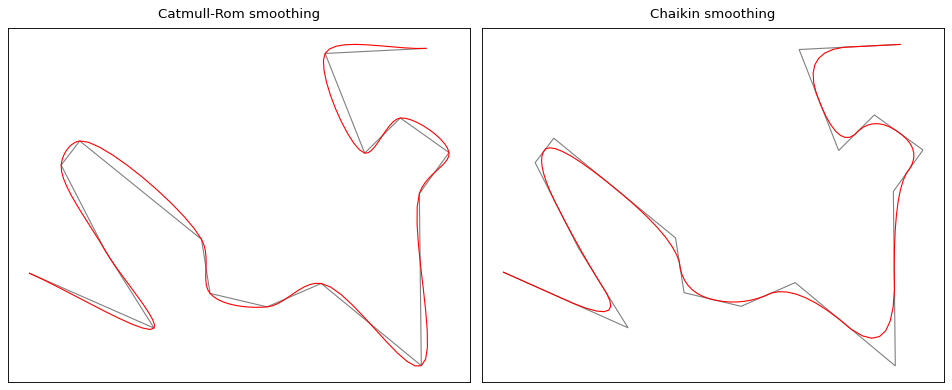
Comparison between Catmull-Rom and Chaikin

Polygons

Buildings

CartAGen also contains algorithms that process any type of polygons, and others specific to some types of map polygons, such as buildings. This section contains only informations related to algorithms that process one polygon at a time. If your buildings seems to be adapted to your current scale, you can still run a squaring algorithm to correct angles that are almost flat, right, or at 45 degrees, using:

• Least square squaring [24]

• Naive squaring [24]

(Source code)

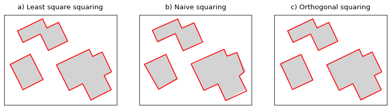
Building squaring algorithms

If you want to modify further the geometry of the building, you can use simplification algorithms, such as:

• Building simplification [25]

(Source code)

Building simplification

The building simplification algorithm is a simple algorithm design to reduce the complexity of buildings by removing edges.

CartAGen contains algorithms designed to process buildings computed from segmentation of aerial or satellite images. Those algorithms can drastically

• Rectangle transformation

• Recursive regression [26] [27]

• Feature Edge Reconstruction (FER) [27]

(Source code)

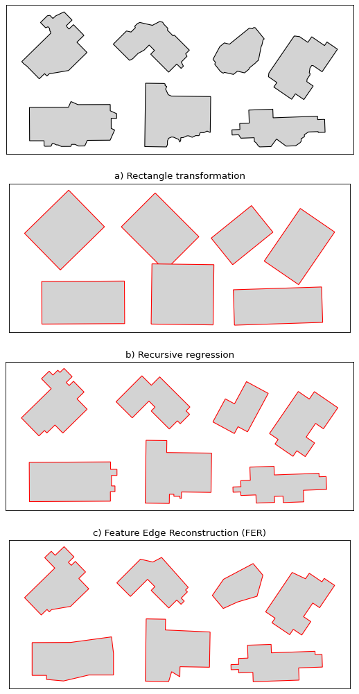
Building regularization algorithms

Recursive regression can be quite destructive and is will always return 45 degrees angles. On the other hand, the rectangle transformation is mostly used inside more complex algorithms, such as AGENT as a possible branch inside a decision tree. Feature edge reconstruction is a complex algorithm with a decision tree that is design to keep the overall shape of the building.

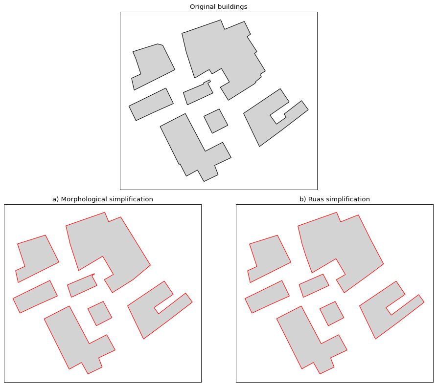
CartAGen also contains algorithms that process several buildings at a time, usually to create amalgamated representation of buildings.

• Building amalgamation [28]

(Source code)

Building amalgamation algorithm

Building blocks

A building block can be defined as several buildings inside the face of a road network, and usually in an urban area to have a high enough density to require generalisation. Different operations can then be applied depending on factors such as the density of buildings and the final scale of the map.

At large scale, maybe we need to keep the individual buildings without modifying their geometry and the space inside the building block is enough for the buildings to be moved. Thus, we can use the random displacement algorithm.

(Source code)

Random displacement of buildings inside the building block

Still at large scale, sometimes there is not enough space inside the building block to move the buildings around. It often is the case in urban areas, where buildings are touching each other. So, you may want to aggregate those buildings into a representation of the building blocks that takes into consideration the shapes of the individual buildings. For that purpose, you can use the morphological amalgamation [29] and recreate the building blocks.

(Source code)

Morphological amalgamation of buildings into building blocks

Urban areas

Sometimes, you will need to generate a representation of an urban area. This can be achieved by representing the extent of the buildings if you consider your buildings as representative of the urban area. This can be done using the algorithm to calculate Boffet area. [30]

(Source code)

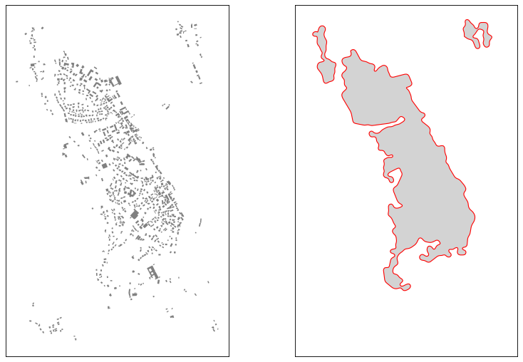
Boffet areas with a small gaussian smoothing applied to the result

Typification

In dense suburban areas, you might want to use typification to enhance the legibility of the map. We currently have two typification algorithms:

• Matching-based typification [31]

• Burghardt-Cecconi Delauney-based typification [32]

(Source code)

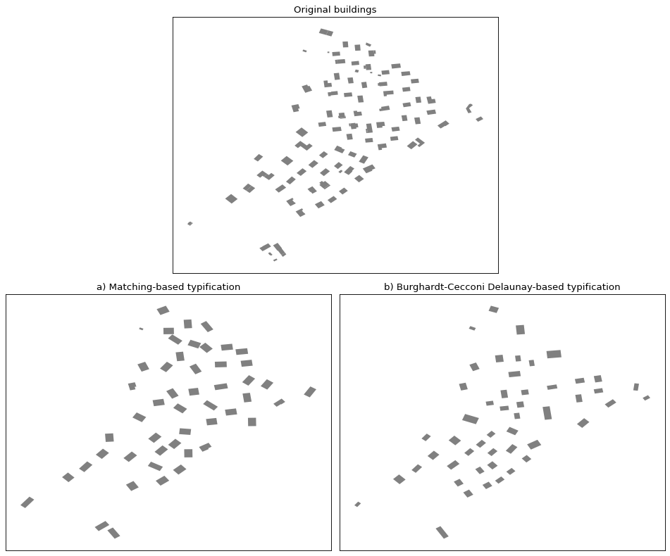
Building typification in dense urban areas

Networks

CartAGen also proposes network-related algorithms intended for the generalisation of different type of artificial or natural linear networks.

Roads

Road networks algorithms are designed to detect or collapse specific road network features such as roundabouts, branching crossroads or dual carriageways. They can be dependent on each other, for example, collapsing roundabouts depends on both roundabout detection and branching crossroads detection to yield better results.

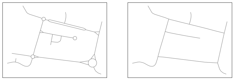
Having that in mind, the following section illustrates an example of a network generalisation workflow using network enrichment functions and collapsing algorithms. Let’s consider the following road network as the base data, which has too much detail for the scale we want.

(Source code)

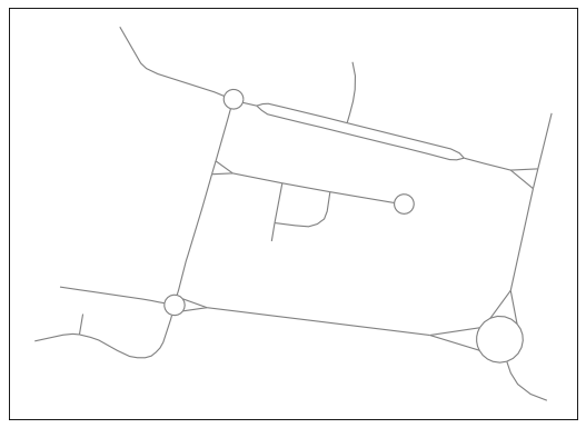
The original road network.

It is advised to make your network planar before using any generalisation algorithms as it will avoid most issues afterwards.

(Source code)

The original network (left) and the network made planar (right). The color are used only on non-planar edges to show their geometries.

Roundabouts and branching crossroads

We can start by using detect_roundabouts followed by detect_branching_crossroads to respectively detect roundabouts and then branching crossroads. We can specify detected roundabouts as an input when detecting branching crossroads, that way, when those two objects are connected, they can be treated as one object when collapsing.

# The variable network is a GeoDataFrame of LineString representing
# the network to generalise
roundabouts = detect_roundabouts(network)
crossroads = detect_branching_crossroads(network, roundabouts)

Then, we can apply collapse_branching_crossroads followed by collapse_roundabouts to collapse those shapes and simplify the network. The order is important as the first will collapse branching crossroads that are not connected to roundabouts, and then collapse roundabouts and mixed objects (roundabouts with incoming branching crossroads).

network = collapse_branching_crossroads(network, crossroads)
network = collapse_roundabouts(network, roundabouts, crossroads)

(Source code)

Collapsing roundabouts (in red) and branching crossroads (in blue) inside the road network.

Dual carriageways

We can now detect dual carriageways using detect_dual_carriageways…

carriageways = detect_dual_carriageways(network)

…and collapse them using collapse_dual_carriageways.

network = collapse_dual_carriageways(network, carriageways)

(Source code)

Collapsing dual carriageways inside the road network.

Dead ends

Now, we can detect dead-ends by using detect_dead_ends. This stage can be deployed at the discretion of the cartographer as it can be used to clean up the network. Here, we used this after collapsing branching crossroads as the dead-end located at the center of the current network would not have been detected. You can read more about how dead-ends are detected in their API reference page.

network = detect_dead_ends(network, True)

Finally, we can eliminate dead-end groups using eliminate_dead_ends that are shorter than 200 meters and simplify long dead-end groups by keeping only the longest path.

network = eliminate_dead_ends(network, 200, keep_longest=True)

(Source code)

Eliminate or simplify dead-end groups (in red) inside the network.

We can then compare our input network and our result to see how the network generalisation simplified the roads layout details in order to represent them at a larger scale. Keep in mind that generalisation of a road network is a complex process and sometimes algorithms can have a hard time finding specific features. For example, you could have a branching crossroad that is not triangular, and thus, it won’t be detected as one. This is a reminder that good generalisation relies on the cartographer’s validation at the end of the process.

(Source code)

The original network (left) and the network after generalisation (right).

Complex junctions

For now, only one algorithm is designed to work on complex junctions, collapse_junctions. It is mostly used on highway interchanges, but it can lead to weird output and may not be suited for every use cases.

(Source code)

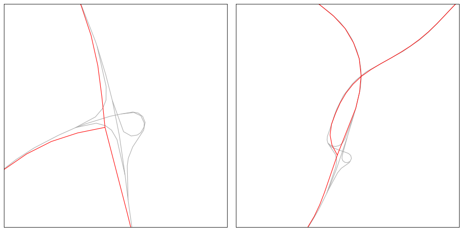
The original network (left) and the network after generalisation (right) and smoothing.

Processes

AGENT

Agent-based generalization follows a step by step, knowledge based approach, which arises from the seminal model from Ruas & Plazanet [33]. The aim is not to find a global solution to generalize the whole map at once, but to identify local situations that require generalization, and try generalization algorithms to improve the legibility of this situation.

This process is a port of the version present in the CartAGen Java application. For a better understanding of the AGENT process, you can refer to Barrault et al. [34], Ruas & Duchêne [35] and Duchêne et al. [36]

Micro-agents

Micro-agents are the simpler kind of agents as they aim at generalising single cartographic features without consideration for their surroundings.

Assuming the variable buildings is a GeoDataFrame of Polygon, we need to loop through buildings and add them as individual agent before generalisation:

import cartagen as c4

agents = []
for i, building in buildings.iterrows():
    # Create the agent
    agent = c4.BuildingAgent(building)

    # Adding a size constraint of 250 square meters to enlarge the building if needed
    size = c4.BuildingSizeConstraint(agent, importance=1, min_area=250)

    # Adding a granularity constraint that will simplify the building if
    # an edge is above the minimum allowed length
    granularity = c4.BuildingGranularityConstraint(agent, importance=1, min_length=6)

    # Adding a squareness constraint to square the building angles if needed
    squareness = c4.BuildingSquarenessConstraint(agent, importance=1)

    agent.constraints.append(size)
    agent.constraints.append(squareness)
    agent.constraints.append(granularity)
    agents.append(agent)

c4.run_agents(agents)

Below is a table representing the different constraints available for the building generalisation using AGENT along with their associated actions.

Building micro constraints

Name	Property	Actions
BuildingSizeConstraint	area	enlarge, delete
BuildingGranularityConstraint	granularity	simplify, simplify to rectangle
BuildingSquarenessConstraint	squareness	squaring

(Source code)

Resulting generalisation using the micro-agents

Least squares-based method

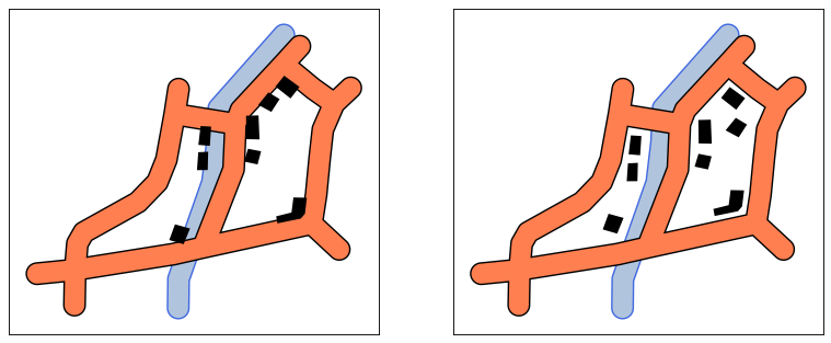
CartAGen also propose a generalisation method based on the method of least squares. This method was proposed by Harrie [37] and relies on the least squares regression to displace every vertexes of every provided objects (points, lines and polygons). Those vertexes can move but they need to respect user-provided constraints. In practice, it iteratively tries to resolve matrice equations until a threshold norm is reached keeping every constraints as satisfied as possible.

Setup

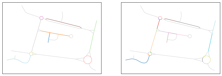
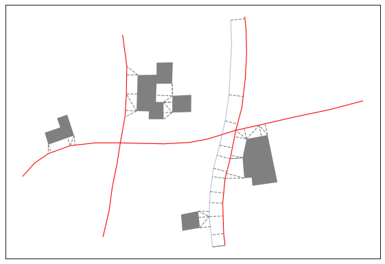
As en example, let’s start with a set of three geographic objects (example in the image below), namely some buildings (in gray), a simple road network (in red) and a river (in blue).

Let’s consider those objects are too close to each other at the scale we want to represent them. We can start by instanciating the least squares method class with default parameters:

ls = cartagen.LeastSquaresMethod()

Constraints

But we also want to specify constraints to maintain some control over the movement of vertexes. Using the following table, we can specify different constraints for the different objects:

Constraints description used by the method of least squares

Constraint	Geometry type	Impact
movement	Point, LineString, Polygon	The object should move as little as possible
stiffness	LineString, Polygon	The internal geometry should be invariant, i.e. the vertexes movement within the same object will try not to move closer or away from each other.
curvature	LineString, Polygon	The curvature of a line or a polygon border should not change, i.e. the angle formed by two connected segments will try not to change.

Having that in mind, we can add the different objects with the constraints properly set. The numbers represent the weight of the constraint. A higher value means the constraint will be more respected during generalisation. So, in the following example, the buildings have a high stiffness which means there shape will tend to stay the same:

ls.add(buildings, movement=2, stiffness=10)
ls.add(roads, movement=2, curvature=5)
ls.add(rivers, movement=2, curvature=5)

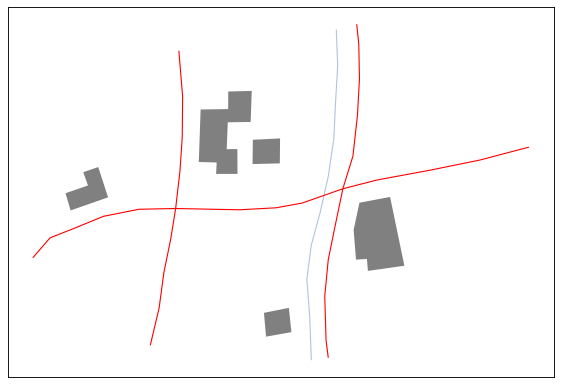
Spatial relationships

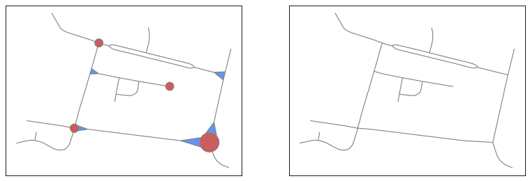
We decided to let users more freedom when setting the spatial conflict constraints. Thus, we can decide the distance and weight of spatial conflicts between each pair of objects we already added. So, we need to provide two matrices: one for the distances between pairs of objects, one for the weight of those spatial constraints.

First, we retrieve the number of objects added for generalisation. This should be 3: buildings, roads, rivers:

d = ls.get_objects_number()

We can then create two numpy arrays of the right shape:

distances = np.zeros((d, d))
spatial_weights = np.zeros((d, d))

We then can populate the new arrays with default distance and weight values:

for i in range(d):
    for j in range(d):
        distances[i][j] = 20
        spatial_weights[i][j] = 5

Those two arrays represent the spatial conflicts and the weight of those conflicts between each pairs of objects. So, by setting a default distance, we will force objects to have at least 20 meters between each other.

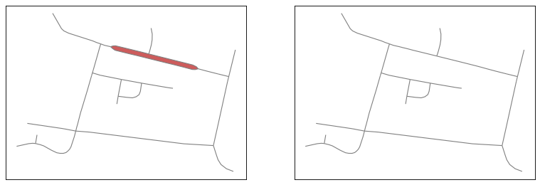
But maybe we want to allow buildings to be closer to each other and further away from the rivers. To change those distances, we can use ls.distances[n][m] where n and m are respectively the index of the pair of object we want to modify in the order we added them. Let’s say we want buildings to be at least at 25 meters from each other, 28 meters from the roads and 30 meters from the rivers, we can do:

distances[0][0] = 25
distances[0][1] = 28
distances[0][2] = 30

The distances variable now return:

[[25. 28. 30.]
 [20. 20. 20.]
 [20. 20. 20.]]

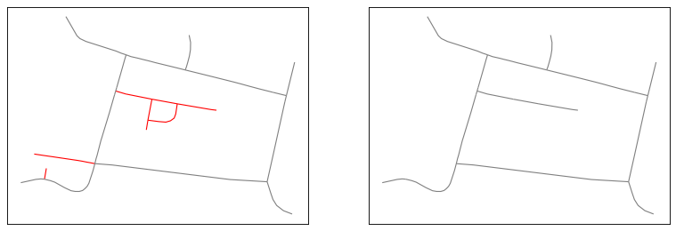
And if we want to increase the weight of the spatial conflict between the roads and the rivers, we can change it this way:

spatial_weights[1][2] = 8

The spatial_weights variable now return:

[[5. 5. 5.]
 [5. 5. 8.]
 [5. 5. 5.]]

Finally, we can add the spatial relationships to the least squares method:

ls.add_spatial_conflicts(distances, spatial_weights)

Results

Finally, we can launch the generalisation that will return a tuple with as many as objects we added:

buildings, roads, rivers = ls.generalise()

(Source code)

Geographic objects before generalisation

(Source code)

Spatial conflicts detected

(Source code)

Results of the generalisation

Bibliography

[1]

Pia Bereuter and Robert Weibel. Quadtree-based algorithms for point data generalisation. In Computer Science. 2012. URL: https://api.semanticscholar.org/CorpusID:268066143.

[2]

Mathias Gröbe and Dirk Burghardt. Scale-dependent point selection methods for web maps. KN - Journal of Cartography and Geographic Information, 71:143 – 154, 2021. URL: https://api.semanticscholar.org/CorpusID:236972402.

[3]

Matt Duckham, Lars Kulik, Mike Worboys, and Antony Galton. Efficient generation of simple polygons for characterizing the shape of a set of points in the plane. Pattern Recognition, 41(10):3224–3236, 2008. URL: https://www.sciencedirect.com/science/article/pii/S0031320308001180, doi:https://doi.org/10.1016/j.patcog.2008.03.023.

[4]

Antony Galton and Matt Duckham. What is the region occupied by a set of points? In International Conference Geographic Information Science. 2006. URL: https://api.semanticscholar.org/CorpusID:18406174.

[5]

Leland Wilkinson and Michael Friendly. The history of the cluster heat map. The American Statistician, 63:179 – 184, 2009. URL: https://api.semanticscholar.org/CorpusID:122792460.

[6] (1,2)

ROBERT BRAINERD MCMASTER. Automated line generalization. Cartographica, 24(2):74–111, 1987. URL: https://doi.org/10.3138/3535-7609-781G-4L20, doi:10.3138/3535-7609-781G-4L20.

[7]

David H. Douglas and Thomas K. Peucker. Algorithms for the reduction of the number of points required to represent a digitized line or its caricature. Cartographica: The International Journal for Geographic Information and Geovisualization, 10(2):112–122, 1973. URL: https://doi.org/10.3138/FM57-6770-U75U-7727, arXiv:https://doi.org/10.3138/FM57-6770-U75U-7727, doi:10.3138/FM57-6770-U75U-7727.

[8]

T. Lang. Rules for robot draughtsmen. Geographical Magazine, 01 1969.

[9]

Zhilin Li and Stan Openshaw. A natural principle for the objective generalization of digital maps. In Computer Science, Geography. 1993. URL: https://api.semanticscholar.org/CorpusID:120732702.

[10]

Paulo Raposo. Scale-specific automated line simplification by vertex clustering on a hexagonal tessellation. Cartography and Geographic Information Science, 40(5):427–443, 2013. URL: https://doi.org/10.1080/15230406.2013.803707, arXiv:https://doi.org/10.1080/15230406.2013.803707, doi:10.1080/15230406.2013.803707.

[11]

K. Reumann and A. Witkam. Optimizing curve segmentation in computer graphics. Proceedings of International Computing Symposium, 01 1974.

[12]

M. Visvalingam and J.D. Whyatt. Line generalization by repeated elimination of points. The Cartographic Journal, 30(1):46–51, 1993. URL: https://www.tandfonline.com/doi/abs/10.1179/000870493786962263, arXiv:https://www.tandfonline.com/doi/pdf/10.1179/000870493786962263, doi:10.1179/000870493786962263.

[13]

James Dougenik. Whirlpool: a geometric processor for polygon coverage data. In Proceedings of Auto-Carto 4. Reston, Virginia, USA, 1979.

[14]

Jean Babaud, Andrew P. Witkin, Michel Baudin, and Richard O. Duda. Uniqueness of the gaussian kernel for scale-space filtering. IEEE Transactions on Pattern Analysis and Machine Intelligence, PAMI-8:26–33, 1986. URL: https://api.semanticscholar.org/CorpusID:18295906.

[15]

Corinne Plazanet. Enrichissement des bases de données géographiques : analyse de la géométrie des objets linéaires pour la généralisation cartographique (application aux routes). PhD thesis, École nationale des sciences géographiques, Marne-la-Vallée, France, 1996. Thèse de doctorat dirigée par Désarménien, Jacques Sciences de l’information géographique Marne-la-Vallée 1996. URL: http://www.theses.fr/1996MARN0001.

[16]

Emmanuel Fritsch. Représentations de la géométrie et des contraintes cartographiques pour la généralisation du linéaire routier. PhD thesis, École nationale des sciences géographiques, Marne-la-Vallée, France, 1998. URL: https://documentation.ensg.eu/index.php?lvl=notice_display&id=45154.

[17]

Dirk Burghardt. Controlled line smoothing by snakes. Geoinformatica, 9(3):237–252, September 2005. URL: https://doi.org/10.1007/s10707-005-1283-3, doi:10.1007/s10707-005-1283-3.

[18]

Gabriel Taubin. Curve and surface smoothing without shrinkage. In Proceedings of IEEE International Conference on Computer Vision, 852–857. 07 1995. doi:10.1109/ICCV.1995.466848.

[19]

J. C. Müller and Wang Zeshen. Area-patch generalisation: a competitive approach. The Cartographic Journal, 29(2):137–144, 1992. URL: https://www.tandfonline.com/doi/abs/10.1179/000870492787859763, doi:10.1179/000870492787859763.

[20]

Edwin E. Catmull and Raphael Rom. A class of local interpolating splines. Computer Aided Geometric Design, pages 317–326, 1974. URL: https://api.semanticscholar.org/CorpusID:118383557.

[21]

Phillip Barry and Ronald Goldman. Recursive evaluation algorithm for a class of catmull-rom splines. In Proceedings of the 15th Annual Conference on Computer Graphics and Interactive Techniques, volume 22, 199–204. 08 1988. doi:10.1145/378456.378511.

[22]

George Merrill Chaikin. An algorithm for high-speed curve generation. Computer Graphics and Image Processing, 3(4):346–349, 1974. URL: https://www.sciencedirect.com/science/article/pii/0146664X74900288, doi:https://doi.org/10.1016/0146-664X(74)90028-8.

[23]

Ling Wu, Jun-Hai Yong, You-Wei Zhang, and Li Zhang. Multi-step subdivision algorithm for chaikin curves. In Jun Zhang, Ji-Huan He, and Yuxi Fu, editors, Computational and Information Science, 1232–1238. Berlin, Heidelberg, 2005. Springer Berlin Heidelberg.

[24] (1,2)

Guillaume Touya and Imran Lokhat. Enhancing building footprints with squaring operations. Journal of Spatial Information Science, December 2016. URL: https://hal.science/hal-02147792, doi:10.5311/JOSIS.2016.13.276.

[25]

Anne Ruas. Modèle de généralisation de données géographiques à base de contraintes et d’autonomie. PhD thesis, École nationale des sciences géographiques, Marne-la-Vallée, France, 1999. Thèse de doctorat dirigée par Désarménien, Jacques Sciences de l’information géographique Marne-la-Vallée 1999. URL: http://www.theses.fr/1999MARN0050.

[26]

Tomás Bayer. Automated building simplification using a recursive approach. In Computer Science, Engineering. 2009. URL: https://api.semanticscholar.org/CorpusID:18911893.

[27] (1,2)

Min Yang, Renwei Zou, Tinghua Ai, and Xiongfeng Yan. Regularizing building outlines extracted from remote sensing images by integrating multiple algorithms. Geocarto International, 2024. URL: https://api.semanticscholar.org/CorpusID:270784716.

[28]

Nicolas Regnauld. Généralisation du bâti: Structure spatiale de type graphe et représentation cartographique. PhD Thesis, Université de Provence, 1998.

[29]

Jonathan Damen, Marc J. van Kreveld, and Bert Spaan. High quality building generalization by extending the morphological operators. In Computer Science. 2008. URL: https://api.semanticscholar.org/CorpusID:218476605.

[30]

Annabelle Boffet. Généralisation cartographique et description des espaces urbains. In Bulletin de l’Association de Géographes Français. 2003. URL: https://api.semanticscholar.org/CorpusID:118066053.

[31]

Hongsheng Li, Qingsheng Guo, and Jiping Liu. Rapid algorithm of building typification in web mapping. In Proceedings of the International Symposium on Spatio-Temporal Modelling. 08 2005. URL: https://api.semanticscholar.org/CorpusID:6031841.

[32]

D. Burghardt and A. Cecconi. Mesh simplification for building typification. International Journal of Geographical Information Science, 21(3):283–298, 2007. URL: https://doi.org/10.1080/13658810600912323, arXiv:https://doi.org/10.1080/13658810600912323, doi:10.1080/13658810600912323.

[33]

A Ruas and C Plazanet. Strategies for automated generalization, in proceedings of the 7 th international symposium on spatial data handling. Advances in GIS Research II, pages 6–1, 1996.

[34]

Mathieu Barrault, Nicolas Regnauld, Cécile Duchêne, Kelvin Haire, Christof Baeijs, Yves Demazeau, Paul Hardy, William A. Mackaness, Anne Ruas, and Robert Weibel. Integrating multi agent, object oriented and algorithmic techniques for improved automoated map generalisation. In Computer Science, Geography. 2001. URL: https://api.semanticscholar.org/CorpusID:42164293.

[35]

Anne Ruas and Cécile Duchêne. Chapter 14 - a prototype generalisation system based on the multi-agent system paradigm. In William A. Mackaness, Anne Ruas, and L. Tiina Sarjakoski, editors, Generalisation of Geographic Information, International Cartographic Association, pages 269–284. Elsevier Science B.V., Amsterdam, 2007. URL: https://www.sciencedirect.com/science/article/pii/B9780080453743500168, doi:https://doi.org/10.1016/B978-008045374-3/50016-8.

[36]

Cécile Duchêne, Guillaume Touya, Patrick Taillandier, Julien Gaffuri, Anne Ruas, and Jérémy Renard. Multi-Agents Systems for Cartographic Generalization: Feedback from Past and On-going Research. Research Report, IGN (Institut National de l’Information Géographique et Forestière) ; LaSTIG, équipe COGIT, January 2018. URL: https://hal.science/hal-01682131.

[37]

Lars Harrie. The constraint method for solving spatial conflicts in cartographic generalization. In Computer Science, Geography. 1999. URL: https://api.semanticscholar.org/CorpusID:62418580.